Machine Learning at SourceClear

As you may know, SourceClear has the world’s most complete, accurate, and up-to-date database of verified vulnerabilities in open-source code. But what’s more important is that more than half of the vulnerabilities in our database are not available anywhere else and have no public disclosures. How do we manage to hunt these vulnerabilities from thousands of open-source libraries? Certainly, it would be too exhausting to manually track and review each library! Today we will walk you through our automated vulnerability identification system that is geared toward tracking large number of projects in real-time using natural language processing and machine learning techniques.

System Overview

The picture below shows the overview of our system. On the left side are our data sources which include commits, JIRA tickets, Bugzilla reports, GitHub issues & pull requests from thousands of open source libraries, and several private mailing lists managed by the security community. For each source, we have built a corresponding trained machine learning model to identify if each item (e.g. a commit or a bug report) from the source is related to a vulnerability or not. The identified vulnerabilities are sent to our vulnerability management platform (called WOPR) for review, after which, they are added to the threat intelligence center.

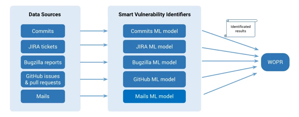
These upstream data sources keep us up-to-date with security-related changes on popular libraries in all the languages we support, like JavaScript, Java, Ruby, Python, PHP, Objective-C and Go lang. The system runs continuously to track potential vulnerabilities from newly updated upstream data sources, enabling us to spot the latest security issues as they are reported in real-time.

How do we iterate on a machine learning model in production?

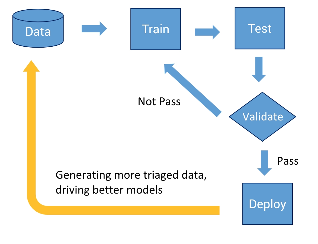
Like most non-trivial machine learning projects, the real challenge is building and maintaining the data pipelines for our models. We usually build an initial usable model and then iterate on it to get better performance. For each data source, we follow the model development cycle shown in the figure below. During the initial training, we experimentally train and test until the results meet our preset target. Then, we put the model into production to validate if the performance matches the test results. After passing the validation, we finally deploy and release the model into production. As we get new data, we retrain and upgrade the existing model if the newly retrained model shows better performance.

Training Pipeline

Now let us introduce our training process. Here we use our data pipeline for commits as an example, but other sources are also handled in a similar fashion.

A glimpse of commits dataset

The first and most crucial part for machine learning is getting the right data. Initially, we pulled all commits from ~2 thousand popular projects. We used regular expression based rules to filter out security-unrelated issues. Using this data, we built the ground truth dataset, where our dedicated security research team labelled all the data and created vulnerability reports. In this way, we collected ~12 thousand security-related commits.

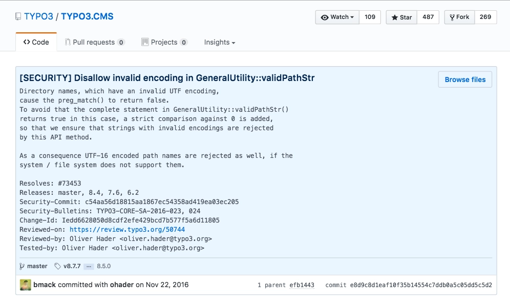
However, only 10.50% of them were related to a vulnerability. In addition to the highly imbalanced nature, the commit messages are unstructured, short, noisy, mixed with urls, abbreviations and variable names, as shown in the commit example below. This, of course, makes the training task quite challenging.

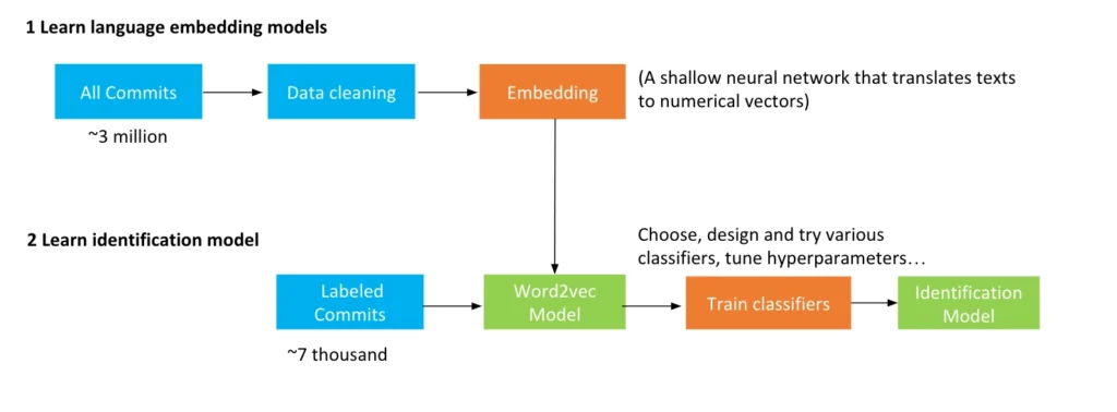
Our initial training pipeline for commits dataset

We use the commit messages as the main feature for the initial training. This requires embedding methods to translate texts in natural languages into numerical vectors. As shown in the training pipeline figure, we built our own word2vec model over 3 million raw commits. The commits messages for training were first fed into the pretrained word2vec model, and then classified to gain the final identification model. We use 2⁄3 of the data for training, and the remaining 1⁄3 for testing.

The second figure above illustrates the workflow of testing a trained vulnerability identification model. The unlabelled commits are mapped into numerical vectors via word2vec model, and then passed into the identification model, where the outputs are the probabilities of being related to vulnerabilities. If the probability of a commit is higher than a predefined threshold, then it is predicted as an vulnerability. The final binary results are compared with the ground truth that are labelled by the security researchers.

Word2vec model over 3 million commits

Now let us take a closer look at the word2vec model constructed with over 3 million commits. Thanks to this model, the performance of our identification model is much better than existing word2vec models based on natural language english text. The word2vec model is trained on a shallow 2-layer neural network to learn vector representation of words based on similarity in context. It contains the dictionaries of {word:vector}. As an example, consider the vector representation of the word xss, and the most similar words:

>>> word2vec['xss']
array([-0.06691808,  0.01889833,  0.08988539,  0.03727728,  0.09463213,
        0.04498576,  0.02401953,  0.01821383, -0.04510168,...., -0.00888534], dtype=float32)
>>> word2vec.most_similar('xss')
[(u'vulnerability', 0.6009132862091064), (u'attacks', 0.5554373860359192), (u'forgery', 0.4951219856739044), (u'spoofing', 0.49092593789100647), (u'dos', 0.4852156937122345), (u'prevention', 0.48259809613227844), (u'clickjacking', 0.48095956444740295), (u'protection', 0.46756529808044434), (u'csrf', 0.457594096660614), (u'vuln', 0.4533842206001282)]

The tuples above show the top 10 most similar words with xss and the corresponding similarity value. The most similar word to xss is vulnerability, followed by attack. As you can see from this example these words are quite similar in the context of security.

Ensemble learning algorithm

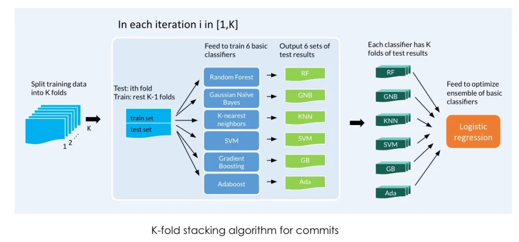
To address the difficulty brought by the highly imbalanced and unstructured nature of the datasets, we designed a K-fold stacking algorithm that ensembles multiple individual classifiers to achieve better identification performance. The algorithm works as follows. It first splits the whole dataset into K folds. For each fold 1 ≤ i ≤ K, the ith part of data is used as the test data, while the rest of the K − 1 parts serve as the training data over which a set of individual classifiers are trained. Therefore after K iterations, each classifier has the full estimation of the whole dataset. Finally the results are fed into an ensemble using a logistic regression.

Observation from Production

We deployed our trained commit model and other models gradually on SourceClear production system. From SourceClear Registry, we can see the value of the models in finding hidden vulnerabilities. The two figures below show the number of public vulnerabilities with CVEs and hidden vulnerabilities without CVEs for JavaScript and the Go language. The ratio of hidden vulnerabilities is as high as 86.51% and 78.20%, respectively. This is especially interesting given that all of the Go-language vulnerabilities were discovered after the deployment of our machine learning models. Simply put, these models were responsible for finding all hidden vulnerabilities in Go.

More ...

If you are interested to know more about our system, its performance, and evaluation, please refer to our recent paper Automated Identification of Security Issues from Commit Messages and Bug Reports [pdf file] that we presented at the joint meeting of European Software Engineering Conference and Symposium on the Foundations of Software Engineering (ESEC/FSE) 2017.